Takata 2025 2D Models with Axionlike Production

Neutrino data for 1-D core-collapse supernova models in the presence of axion-like particles.

The reference article is Progenitor dependence of neutrino-driven supernova explosions with the aid of heavy axionlike particles by T. Takata et al., Phys. Rev. D 111:103028, 2025.

The following models are supported:

ALP parameters and progenitor masses simulated

Progenitor mass [Msun]	Axion mass [MeV]	Axion-photon coupling [1e-10/GeV]
11.2	0, 40, 100, 150, 200, 300, 400, 600, 800	0, 2, 4, 6, 8, 10
20	0, 40, 100, 150, 200, 300, 400, 600, 800	0, 2, 4, 6, 8, 10
25	0, 40, 100, 150, 200, 300, 400, 600, 800	0, 2, 4, 6, 8, 10

from snewpy.neutrino import Flavor
from snewpy.models.ccsn import Takata_2025

from astropy import units as u

from scipy.interpolate import PchipInterpolator

import numpy as np
import matplotlib as mpl
import matplotlib.pyplot as plt

mpl.rc('font', size=16)

Initialize the 2D models

Use the param property of the model class to see the available parameters. Models are initialized using the axion_mass and axion_coupling parameters.

Takata_2025.param

{'progenitor_mass': <Quantity [11.2, 20. , 25. ] solMass>,
 'axion_mass': <Quantity [  0.,  40., 100., 150., 200., 300., 400., 600., 800.] MeV>,
 'axion_coupling': <Quantity [ 0.,  4.,  6.,  8., 10.] 1e-10 / GeV>}

The model with axion_mass=0 and axion_coupling=0 is a standard simulation with no ALP production.

We’ll use the model with a 25 M\(_\odot\) progenitor.

pmass = 25*u.Msun
model_std = Takata_2025(axion_mass=0, axion_coupling=0, progenitor_mass=pmass)
model_std.metadata

{'Progenitor mass': <Quantity 25. solMass>,
 'Axion mass': 0,
 'Axion coupling': <Quantity 0. 1e-10 / GeV>}

# Initialize a handful of axion models.
models = {}
for (am, ac) in ((40*u.MeV, 4e-10/u.GeV), (100*u.MeV, 6e-10/u.GeV), (200*u.MeV, 6e-10/u.GeV), (300*u.MeV, 8e-10/u.GeV), (400*u.MeV, 10e-10/u.GeV), (600*u.MeV, 6e-10/u.GeV)):
    models[(am,ac)] = Takata_2025(axion_mass=am, axion_coupling=ac, progenitor_mass=pmass)

models

{(<Quantity 40. MeV>,
  <Quantity 4.e-10 1 / GeV>): Takata_2025 Model: 25_040_04.dat
 Progenitor mass  : 25.0 solMass
 Axion mass       : 40.0 MeV
 Axion coupling   : 4.0 1e-10 / GeV,
 (<Quantity 100. MeV>,
  <Quantity 6.e-10 1 / GeV>): Takata_2025 Model: 25_100_06.dat
 Progenitor mass  : 25.0 solMass
 Axion mass       : 100.0 MeV
 Axion coupling   : 6.0 1e-10 / GeV,
 (<Quantity 200. MeV>,
  <Quantity 6.e-10 1 / GeV>): Takata_2025 Model: 25_200_06.dat
 Progenitor mass  : 25.0 solMass
 Axion mass       : 200.0 MeV
 Axion coupling   : 6.0 1e-10 / GeV,
 (<Quantity 300. MeV>,
  <Quantity 8.e-10 1 / GeV>): Takata_2025 Model: 25_300_08.dat
 Progenitor mass  : 25.0 solMass
 Axion mass       : 300.0 MeV
 Axion coupling   : 8.0 1e-10 / GeV,
 (<Quantity 400. MeV>,
  <Quantity 1.e-09 1 / GeV>): Takata_2025 Model: 25_400_10.dat
 Progenitor mass  : 25.0 solMass
 Axion mass       : 400.0 MeV
 Axion coupling   : 10.0 1e-10 / GeV,
 (<Quantity 600. MeV>,
  <Quantity 6.e-10 1 / GeV>): Takata_2025 Model: 25_600_06.dat
 Progenitor mass  : 25.0 solMass
 Axion mass       : 600.0 MeV
 Axion coupling   : 6.0 1e-10 / GeV}

Plot Model Luminosities

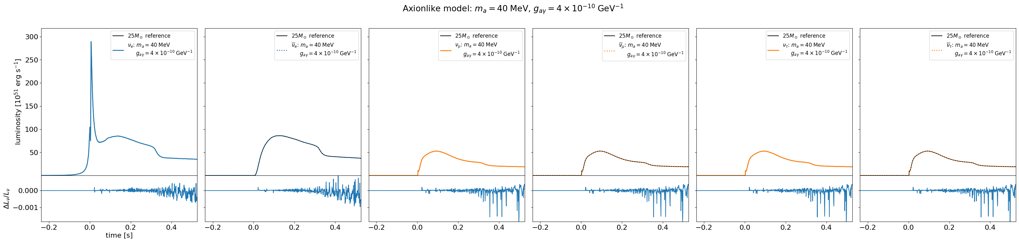
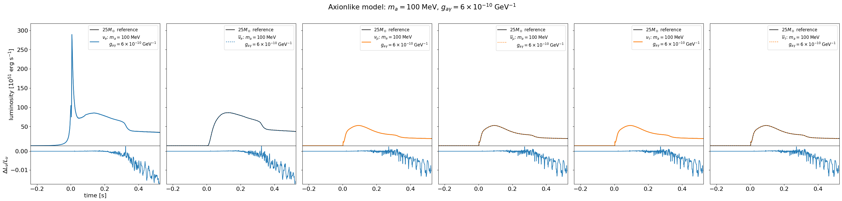
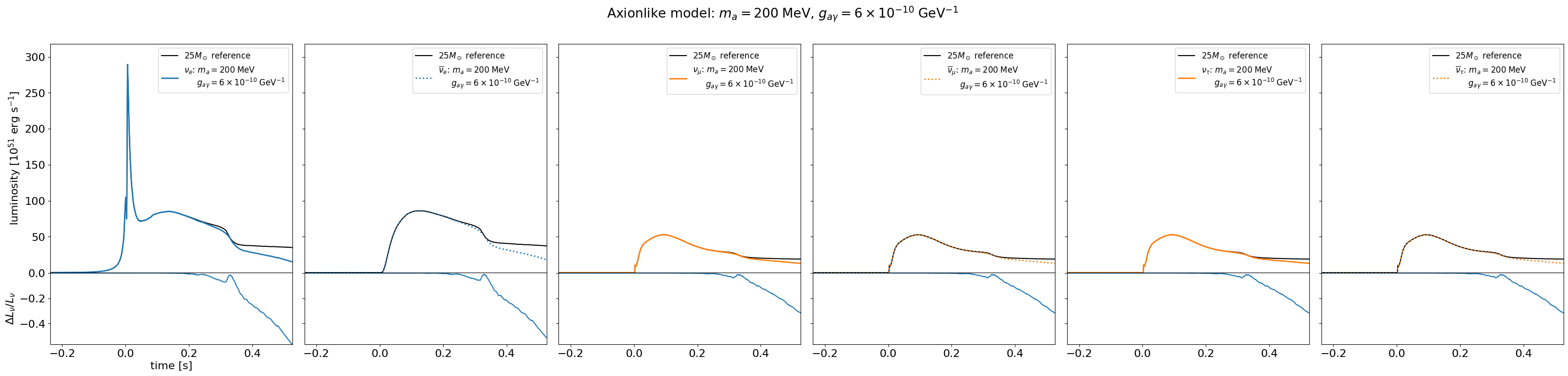
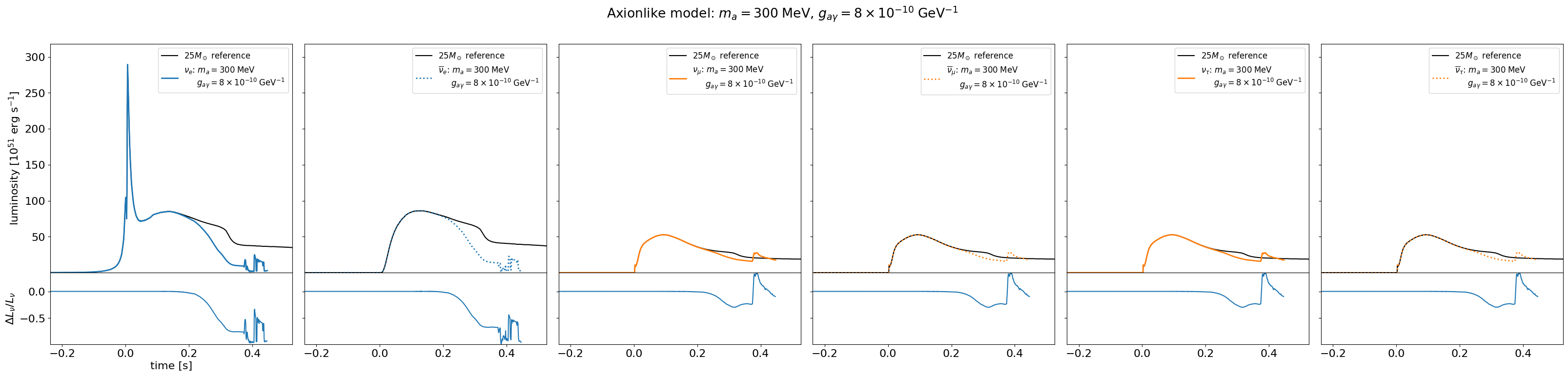
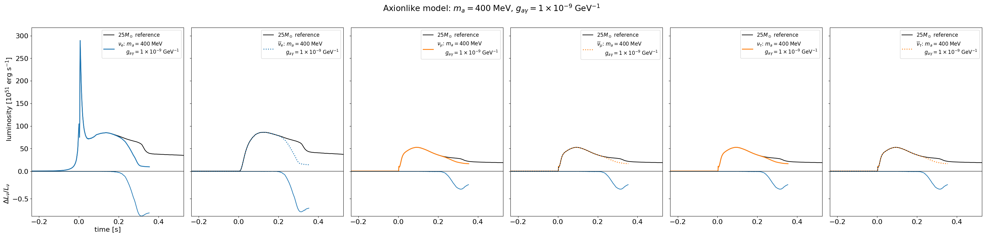
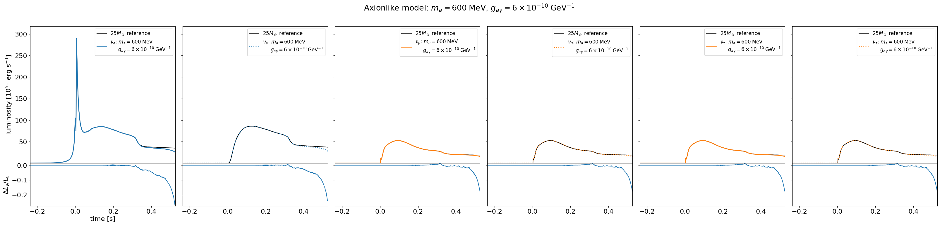
Compare axion model luminosity to the standard 2D simulation.

Higher mass models with stronger coupling constants should produce a decrease in neutrino luminosity at all flavors relative to the reference simulation.

model_std.metadata["Progenitor mass"].to_value("Msun")

np.float64(25.0)

for (m,c), model in models.items():

    fig, axes = plt.subplots(2, 6, figsize=(40, 8), sharex=True,
                         gridspec_kw={'height_ratios':[3.2,1], 'hspace':0, 'wspace':0.05})

    Lmin,  Lmax  = 1e99, -1e99
    dLmin, dLmax = 1e99, -1e99

    for j, (flavor) in enumerate(Flavor):
        ax = axes[0][j]

        ax.plot(model_std.time, model_std.luminosity[flavor]/1e51, 'k', label=rf'${{{model_std.metadata["Progenitor mass"].to_value("Msun"):g}}}M_\odot$ reference')  # Report luminosity in [foe/s]
        Lmin = np.minimum(Lmin, np.min(model_std.luminosity[flavor].to_value('1e51 erg/s')))
        Lmax = np.maximum(Lmax, np.max(model_std.luminosity[flavor].to_value('1e51 erg/s')))

        modlabel = rf"{flavor.to_tex()}: $m_a=${m.to_string(format='latex_inline')}" + "\n" + rf"     $g_{{a\gamma}}=${c.to_string(format='latex_inline')}"
        ax.plot(model.time, model.luminosity[flavor]/1e51,  # Report luminosity in units foe/s
                label=modlabel,
                color='C0' if flavor.is_electron else 'C1',
                ls='-' if flavor.is_neutrino else ':',
                lw=2)
        if j==0:
            ax.set(ylabel=r'luminosity [$10^{51}$ erg s$^{-1}$]')

        ax.legend(fontsize=12)
        ax.set(xlim=(model_std.time[0].to_value('s'), model_std.time[-1].to_value('s')))

        ax = axes[1][j]
        tmin = np.maximum(model.time[0], model_std.time[0]).to_value('s')
        tmax = np.minimum(model.time[-1], model_std.time[-1]).to_value('s')
        times = np.arange(tmin, tmax, 0.001)*u.s

        Lstd = PchipInterpolator(model_std.time, model_std.luminosity[flavor].to_value('1e51 erg/s'))
        Lstd_t = Lstd(times)
        select = Lstd_t != 0

        Lmod = PchipInterpolator(model.time, model.luminosity[flavor].to_value('1e51 erg/s'))
        Lmod_t = Lmod(times)
        dL = (Lmod_t[select] - Lstd_t[select]) / Lstd_t[select]

        dLmin = np.minimum(dLmin, np.min(dL))
        dLmax = np.maximum(dLmax, np.max(dL))

        ax.plot(times[select], dL)
        if j==0:
            ax.set(xlabel='time [s]',
                   ylabel=r'$\Delta L_\nu/L_\nu$')

    for j in range(6):
        axes[0][j].set(ylim=(Lmin, 1.1*Lmax))
        axes[1][j].set(ylim=(dLmin, dLmax))
        if j > 0:
            axes[0][j].set_yticklabels([])
            axes[1][j].set_yticklabels([])

    fig.suptitle(rf"Axionlike model: $m_a=${m.to_string(format='latex_inline')}, $g_{{a\gamma}}=${c.to_string(format='latex_inline')}")

Plot Model Spectra

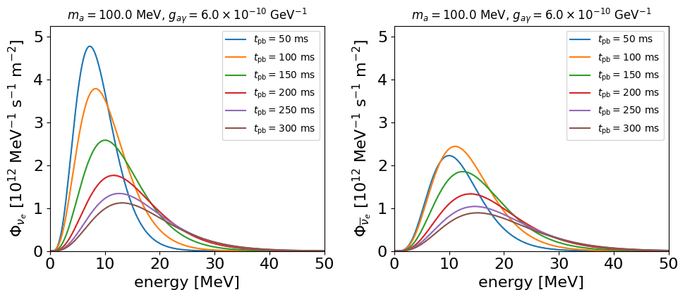
Plot model spectra for the baseline model and a few of the alternative models for several times. Assume the progenitor is at a distance of 1 kpc.

t = np.arange(0.05, 0.35, 0.05) * u.s
E = np.arange(0, 50.1, 0.1) * u.MeV
d = 1*u.kpc

Compare Baseline Model to 100 MeV ALP

Show the spectra from the ALP model at several times. The baseline model (no ALP) spectra are drawn as dashed lines.

nt = t.shape[0]

fig, axes = plt.subplots(1,2, figsize=(10,4.5), sharex=True, tight_layout=True)

fmin, fmax = 0, -1e99

for fl in (Flavor.NU_E, Flavor.NU_E_BAR):
    ax = axes[fl]

    for j in np.arange(nt):
        color = None
        for i, model in enumerate([model_std, models[(100*u.MeV, 6e-10/u.GeV)]]):
            d2fdEdt = model.get_flux(t, E, d)
            dfdE = d2fdEdt.array[fl, j, :].to_value('1e12/(MeV s cm2)')
            fmax = np.maximum(fmax, np.max(dfdE))
            ls = '--' if i == 0 else '-'
            label = None if i == 0 else rf'$t_\text{{pb}}={t[j].to_value("ms"):g}$ ms'
            width = 1 if i==0 else 1.5
            line, = ax.plot(E, dfdE, label=label, ls=ls, lw=width, color=color)
            color = line.get_color()

    ax.set(xlim=E[[0,-1]].to_value(),
           xlabel='energy [MeV]',
           ylim=(fmin, 1.1*fmax),
           ylabel=rf'$\Phi_{{{fl.to_tex()[1:-1]}}}$ [$10^{{12}}$ MeV$^{{-1}}$ s$^{{-1}}$ m$^{{-2}}$]',
          )
    ax.set_title(rf'$m_a=\text{{{model.metadata["Axion mass"]}}}$, $g_{{a\gamma}}={model.metadata["Axion coupling"].to_value("1e-10/GeV")}\times10^{{-10}}$ GeV$^{{-1}}$', fontsize=12)

    ax.legend(loc='upper right', fontsize=10)

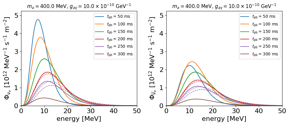
Compare Baseline Model to 400 MeV ALP

Show the spectra from the ALP model at several times. The baseline model (no ALP) spectra are drawn as dashed lines.

nt = t.shape[0]

fig, axes = plt.subplots(1,2, figsize=(10,4.5), sharex=True, tight_layout=True)

fmin, fmax = 0, -1e99

for fl in (Flavor.NU_E, Flavor.NU_E_BAR):
    ax = axes[fl]

    for j in np.arange(nt):
        color = None
        for i, model in enumerate([model_std, models[(400*u.MeV, 10e-10/u.GeV)]]):
            d2fdEdt = model.get_flux(t, E, d)
            dfdE = d2fdEdt.array[fl, j, :].to_value('1e12/(MeV s cm2)')
            fmax = np.maximum(fmax, np.max(dfdE))
            ls = '--' if i == 0 else '-'
            label = None if i == 0 else rf'$t_\text{{pb}}={t[j].to_value("ms"):g}$ ms'
            width = 1 if i==0 else 1.5
            line, = ax.plot(E, dfdE, label=label, ls=ls, lw=width, color=color)
            color = line.get_color()

    ax.set(xlim=E[[0,-1]].to_value(),
           xlabel='energy [MeV]',
           ylim=(fmin, 1.1*fmax),
           ylabel=rf'$\Phi_{{{fl.to_tex()[1:-1]}}}$ [$10^{{12}}$ MeV$^{{-1}}$ s$^{{-1}}$ m$^{{-2}}$]',
          )
    ax.set_title(rf'$m_a=\text{{{model.metadata["Axion mass"]}}}$, $g_{{a\gamma}}={model.metadata["Axion coupling"].to_value("1e-10/GeV")}\times10^{{-10}}$ GeV$^{{-1}}$', fontsize=12)

    ax.legend(loc='upper right', fontsize=10)