Fornax 2024 Models

CCSN neutrino estimates from 25 late-time 3D simulations using the Fornax code. Simulation data are available on this page and this GitHub repository, and documented in the following publications:

• The Gravitational-Wave Signature of Core-Collapse Supernovae by David Vartanyan, Adam Burrows, Tianshu Wang, Matthew S.B. Coleman, and Christopher White Phys. Rev. D 107:103015, 2023.

• Physical Correlations and Predictions Emerging from Modern Core-collapse Supernova Theory by Adam Burrows, Tianshu Wang, and David Vartanyan, Astrophys. J. Lett. 964:16, 2024.

• Gravitational-wave and Gravitational-wave Memory Signatures of Core-collapse Supernovae by Lyla Choi, Adam Burrows, and David Vartanyan, Astrophys. J. 975:12, 2024.

Note that as of June 2026, only the angle-averaged fluxes are available through snewpy.

from snewpy.neutrino import Flavor
from snewpy.models.ccsn import Fornax_2024

from astropy import units as u
from glob import glob

import matplotlib as mpl
import matplotlib.pyplot as plt
import numpy as np

mpl.rc('font', size=16)

Initialize Models

To start, let’s see what progenitors are available for the Fornax_2021 model. We can use the param property to view all physics parameters and their possible values:

Fornax_2024.param

{'progenitor_mass': <Quantity [  8.1 ,   9.  ,   9.25,   9.5 ,   9.6 ,  11.  ,  12.25,  14.  ,
             15.01,  16.5 ,  16.  ,  17.  ,  18.  ,  18.5 ,  19.  ,  19.56,
             20.  ,  21.68,  23.  ,  24.  ,  25.  ,  40.  ,  60.  , 100.  ] solMass>}

We’ll initialise some of these progenitors and plot the luminosity of different neutrino flavors for two of them. (Note that the Fornax_2021 simulations didn’t distinguish between \(\nu_x\) and \(\bar{\nu}_x\), so both have the same luminosity.) If this is the first time you’re using a progenitor, snewpy will automatically download the required data files for you.

models = {}
for m in Fornax_2024.param['progenitor_mass'].value[::2]:
    # Initialise every second progenitor
    models[m] = Fornax_2024(progenitor_mass=m*u.solMass)

models[18.]

Fornax_2024 Model

Parameter	Value
Progenitor mass	\(18\) \(\mathrm{M_{\odot}}\)
Black hole	False
PNS mass	\(1.51\) \(\mathrm{M_{\odot}}\)

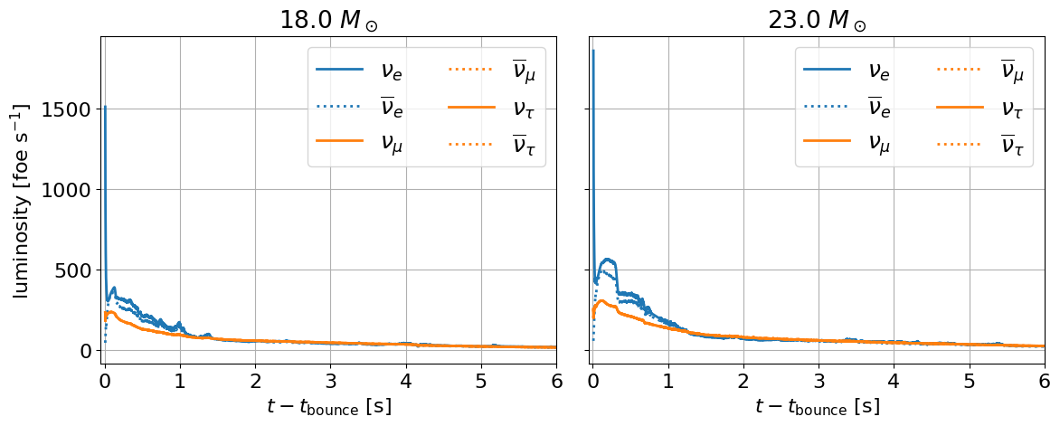
fig, axes = plt.subplots(1, 2, figsize=(12, 5), sharex=True, sharey=True, tight_layout=True)

for i, model in enumerate([models[18.], models[23.]]):
    ax = axes[i]
    for flavor in Flavor:
        ax.plot(model.time, model.luminosity[flavor]/1e51,  # Report luminosity in units foe/s
                label=flavor.to_tex(),
                color='C0' if flavor.is_electron else 'C1',
                ls='-' if flavor.is_neutrino else ':',
                lw=2)
    ax.set(xlim=(-0.05, 6.0),
           xlabel=r'$t-t_{\rm bounce}$ [s]',
           title=r'{} $M_\odot$'.format(model.metadata['Progenitor mass'].value))
    ax.grid()
    ax.legend(loc='upper right', ncol=2, fontsize=18)

axes[0].set(ylabel=r'luminosity [foe s$^{-1}$]');

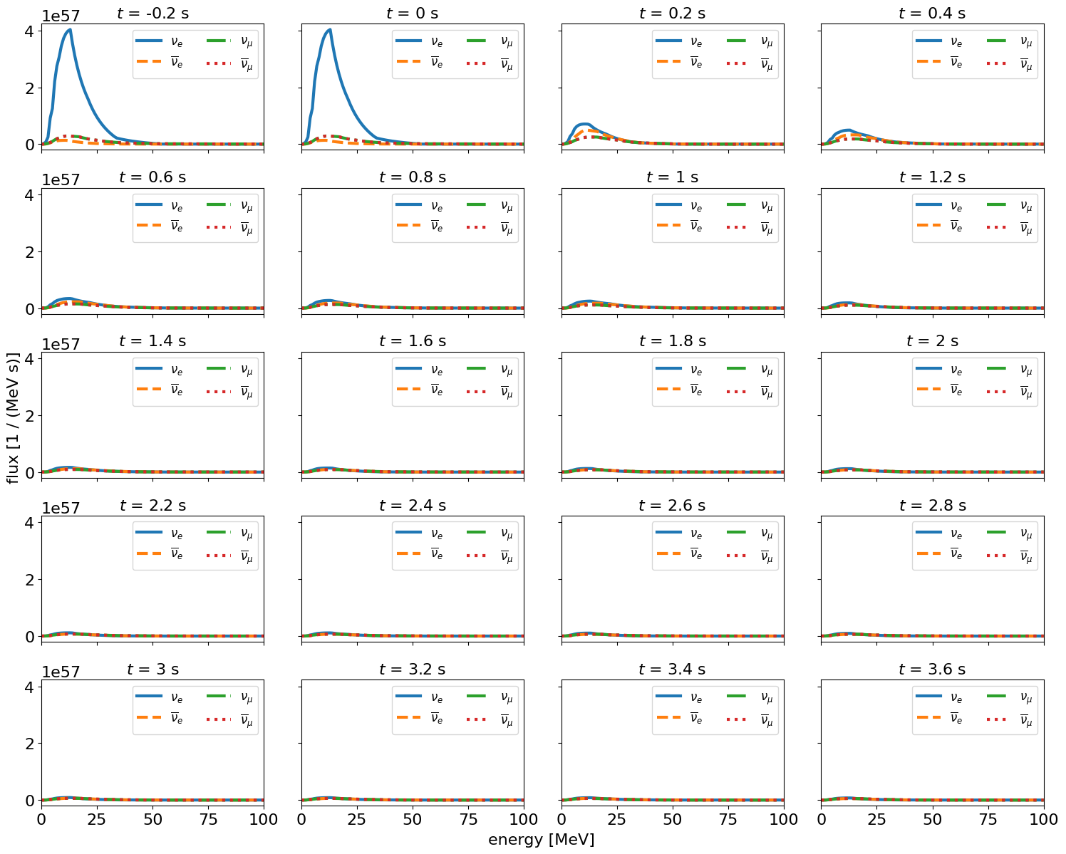
Spectra of All Flavors vs. Time for the \(18M_{\odot}\) Model

Use Default Linear Interpolation in Flux Retrieval

model = models[18.]  # Use the 18 solar mass model

times = np.arange(-0.2, 3.8, 0.2) * u.s
E = np.arange(0, 101, 1) * u.MeV

fig, axes = plt.subplots(5,4, figsize=(15,12), sharex=True, sharey=True, tight_layout=True)

linestyles = ['-', '--', '-.', ':']

spectra = model.get_initial_spectra(times, E)

for i, ax in enumerate(axes.flatten()):
    for line, flavor in zip(linestyles, Flavor):
        ax.plot(E, spectra[flavor,i].array.squeeze(), lw=3, ls=line, label=flavor.to_tex())
    ax.set(xlim=(0,100))
    ax.set_title('$t$ = {:g}'.format(times[i]), fontsize=16)
    ax.legend(loc='upper right', ncol=2, fontsize=12)

fig.text(0.5, 0., 'energy [MeV]', ha='center')
fig.text(0., 0.5, f'flux [{spectra[Flavor.NU_E].unit}]', va='center', rotation='vertical');

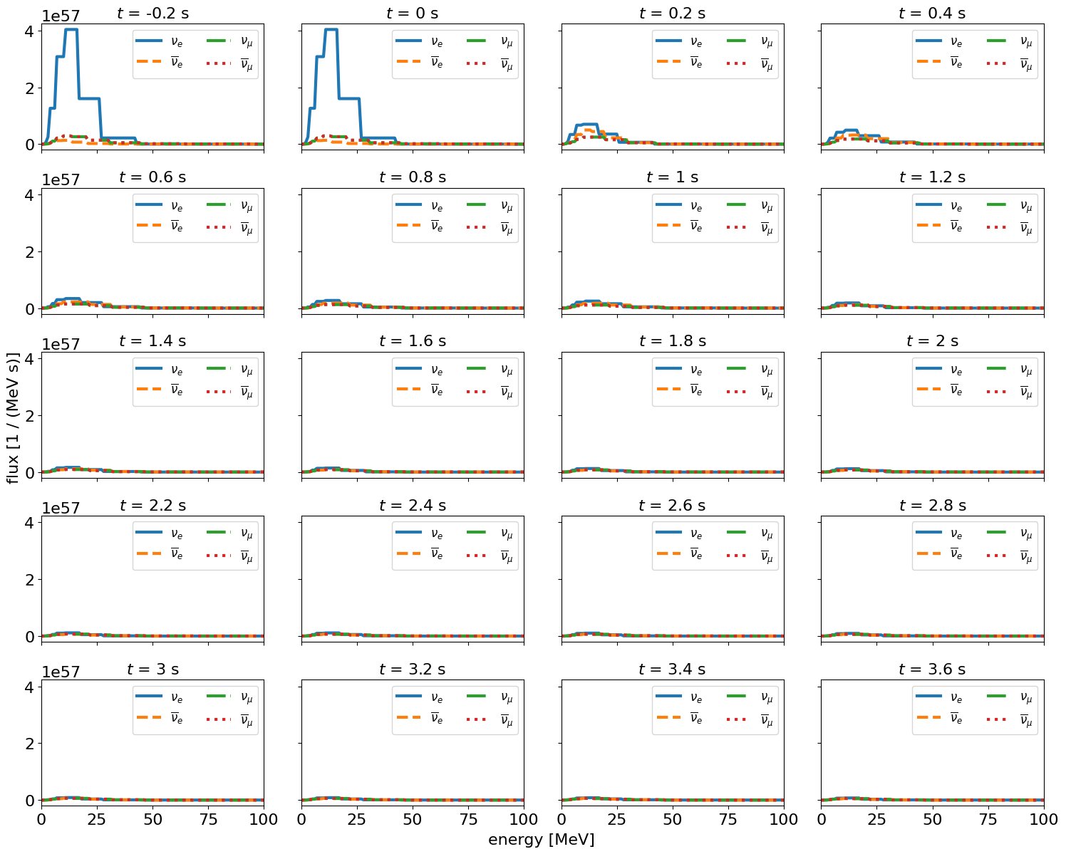
Use Nearest-Bin “Interpolation” in Flux Retrieval

model = models[18.]  # Use the 18 solar mass model

times = np.arange(-0.2, 3.8, 0.2) * u.s
E = np.arange(0, 101, 1) * u.MeV

fig, axes = plt.subplots(5,4, figsize=(15,12), sharex=True, sharey=True, tight_layout=True)

linestyles = ['-', '--', '-.', ':']

model.interpolation='nearest'
spectra = model.get_initial_spectra(times, E)

for i, ax in enumerate(axes.flatten()):
    for line, flavor in zip(linestyles, Flavor):
        ax.plot(E, spectra[flavor,i].array.squeeze(), lw=3, ls=line, label=flavor.to_tex())
    ax.set(xlim=(0,100))
    ax.set_title('$t$ = {:g}'.format(times[i]), fontsize=16)
    ax.legend(loc='upper right', ncol=2, fontsize=12)

fig.text(0.5, 0., 'energy [MeV]', ha='center')
fig.text(0., 0.5, f'flux [{spectra[Flavor.NU_E].unit}]', va='center', rotation='vertical');

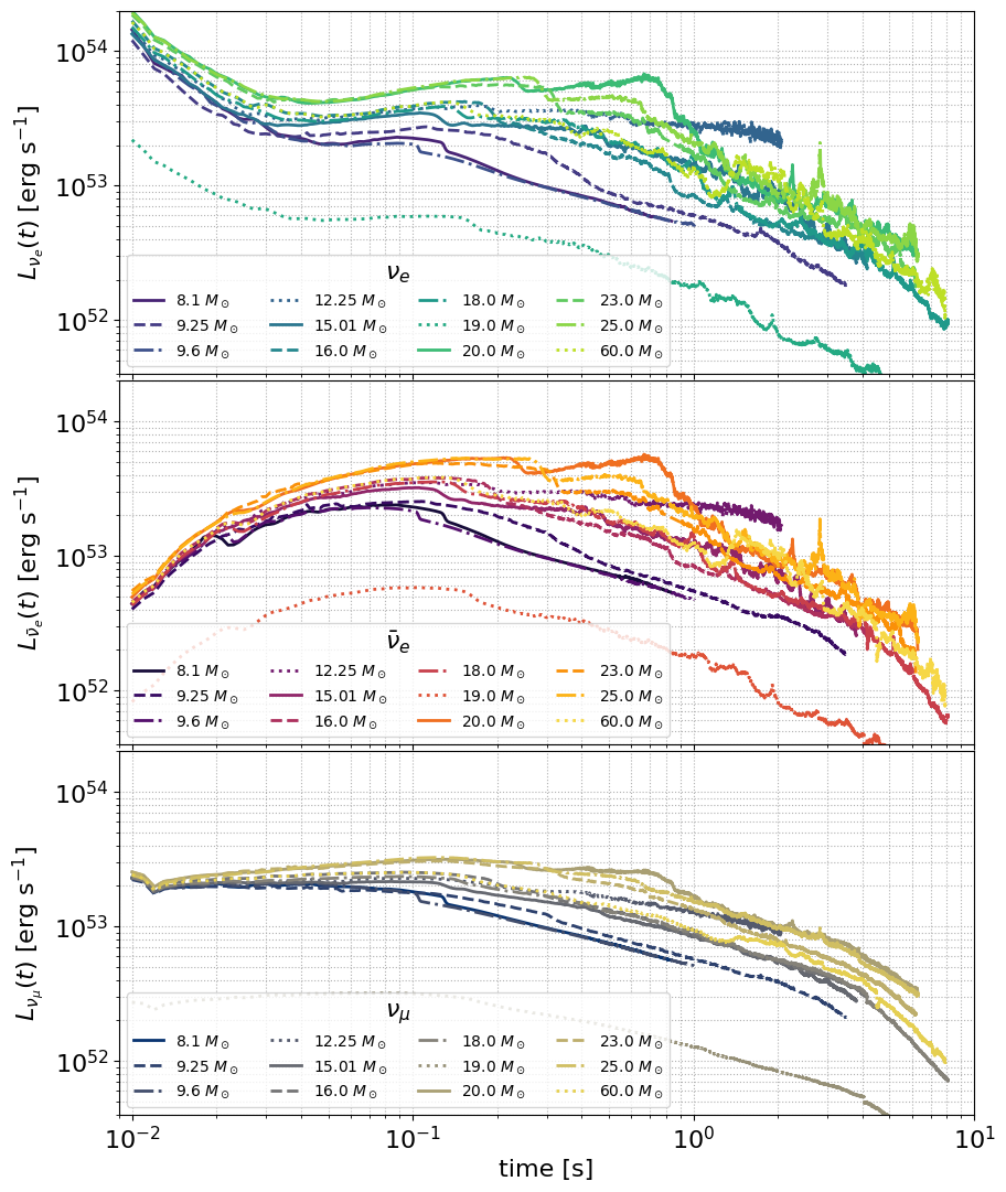
Progenitor Mass Dependence

Luminosity vs. Time for a Selected List of Progenitor Masses

Plot \(L_{\nu_{e}}(t)\) for a selection of progenitor masses to observe the dependence of the emission on mass.

fig, axes = plt.subplots(3,1, figsize=(10,13), sharex=True, sharey=True,
                         gridspec_kw = {'hspace':0.02})

colors0 = mpl.cm.viridis(np.linspace(0.1,0.9, len(models)))
colors1 = mpl.cm.inferno(np.linspace(0.1,0.9, len(models)))
colors2 = mpl.cm.cividis(np.linspace(0.1,0.9, len(models)))

linestyles = ['-', '--', '-.', ':']

for i, model in enumerate(models.values()):
    ax = axes[0]
    flavor = Flavor.NU_E
    ax.plot(model.time, model.luminosity[flavor], lw=2, color=colors0[i], ls=linestyles[i%4],
            label=rf'${model.progenitor_mass}~M_\odot$')
    ax.set(xscale='log',
           xlim=(9e-3, 10),
           yscale='log',
           ylim=(0.4e52, 2e54),
           ylabel=r'$L_{\nu_e}(t)$ [erg s$^{-1}$]')
    ax.grid(ls=':', which='both')
    ax.legend(ncol=4, fontsize=10, title=r'$\nu_e$');

    ax = axes[1]
    flavor = Flavor.NU_E_BAR
    ax.plot(model.time, model.luminosity[flavor], lw=2, color=colors1[i], ls=linestyles[i%4],
        label=rf'${model.progenitor_mass}~M_\odot$')
    ax.set(ylabel=r'$L_{\bar{\nu}_e}(t)$ [erg s$^{-1}$]')
    ax.grid(ls=':', which='both')
    ax.legend(ncol=4, fontsize=10, title=r'$\bar{\nu}_e$');

    ax = axes[2]
    flavor = Flavor.NU_MU
    ax.plot(model.time, model.luminosity[flavor], lw=2, color=colors2[i], ls=linestyles[i%4],
        label=rf'${model.progenitor_mass}~M_\odot$')
    ax.set(xlabel='time [s]',
           ylabel=r'$L_{\nu_\mu}(t)$ [erg s$^{-1}$]')
    ax.grid(ls=':', which='both')
    ax.legend(ncol=4, fontsize=10, title=r'$\nu_\mu$');

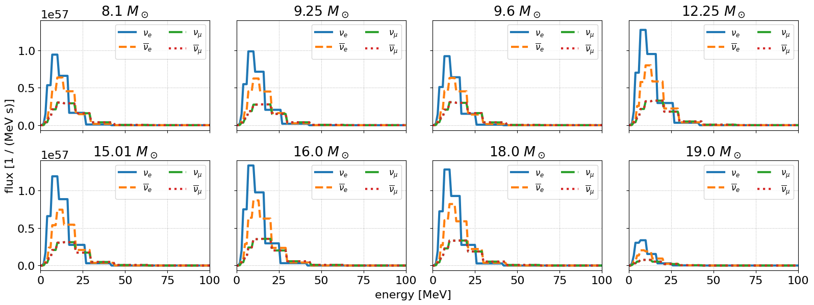
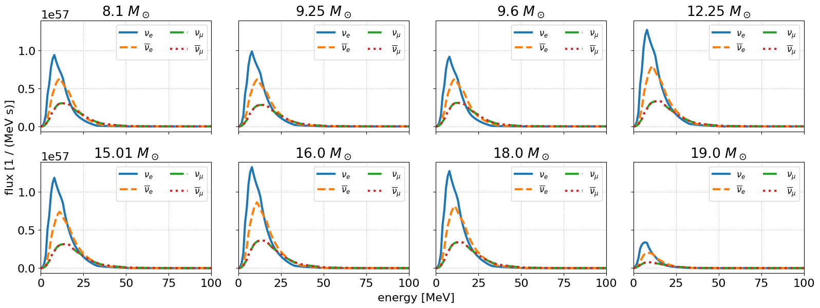
Progenitor Dependence of Spectra at 70 ms

Use Default Linear Interpolation in Flux Retrieval

t = 70*u.ms
E = np.arange(0, 101, 1) * u.MeV

fig, axes = plt.subplots(2,4, figsize=(16,6), sharex=True, sharey=True, tight_layout=True)

linestyles = ['-', '--', '-.', ':']
for model, ax in zip(models.values(), axes.flatten()):
    model.interpolation='linear'
    spectra = model.get_initial_spectra(t, E)
    for line, flavor in zip(linestyles, Flavor):
        ax.plot(E, spectra[flavor,0].array.squeeze(), lw=3, ls=line, label=flavor.to_tex())
    ax.set(xlim=(0,100))
    ax.set_title(rf'${model.progenitor_mass}~M_\odot$')
    ax.legend(loc='upper right', ncol=2, fontsize=12)
    ax.grid(ls=':')

fig.text(0.5, 0., 'energy [MeV]', ha='center')
fig.text(0., 0.5, f'flux [{spectra[Flavor.NU_E].unit}]', va='center', rotation='vertical');

Use Nearest-Bin “Interpolation” in Flux Retrieval

t = 70*u.ms
E = np.arange(0, 101, 1) * u.MeV

fig, axes = plt.subplots(2,4, figsize=(16,6), sharex=True, sharey=True, tight_layout=True)

linestyles = ['-', '--', '-.', ':']
for model, ax in zip(models.values(), axes.flatten()):
    model.interpolation='nearest'
    spectra = model.get_initial_spectra(t, E)
    for line, flavor in zip(linestyles, Flavor):
        ax.plot(E, spectra[flavor,0].array.squeeze(), lw=3, ls=line, label=flavor.to_tex())
    ax.set(xlim=(0,100))
    ax.set_title(rf'${model.progenitor_mass}~M_\odot$')
    ax.legend(loc='upper right', ncol=2, fontsize=12)
    ax.grid(ls=':')

fig.text(0.5, 0., 'energy [MeV]', ha='center')
fig.text(0., 0.5, f'flux [{spectra[Flavor.NU_E].unit}]', va='center', rotation='vertical');